Bias-Variance Tradeoff, Explained: A Visual Guide with Code Examples for Beginners

MODEL EVALUATION & OPTIMIZATION

How underfitting and overfitting fight over your models

Every time someone builds a prediction model, they face these classic problems: underfitting and overfitting. The model cannot be too simple, yet it also cannot be too complex. The interaction between these two forces is known as the bias-variance tradeoff, and it affects every predictive model out there.

The thing about this topic of “bias-variance tradeoff” is that whenever you try to look up these terms online, you’ll find lots of articles with these perfect curves on graphs. Yes, they explain the basic idea — but they miss something important: they focus too much on theory, not enough on real-world problems, and rarely show what happens when you work with actual data.

Here, instead of theoretical examples, we’ll work with a real dataset and build actual models. Step by step, we’ll see exactly how models fail, what underfitting and overfitting look like in practice, and why finding the right balance matters. Let’s stop this fight between bias and variance, and find a fair middle ground.

What is Bias-Variance Tradeoff?

Before we start, to avoid confusion, let’s make things clear about the terms bias and variance that we are using here in machine learning. These words get used differently in many places in math and data science.

Bias can mean several things. In statistics, it means how far off our calculations are from the true answer, and in data science, it can mean unfair treatment of certain groups. Even in the for other part of machine learning which in neural networks, it’s a special number that helps the network learn

Variance also has different meanings. In statistics, it tells us how spread out numbers are from their average and in scientific experiments, it shows how much results change each time we repeat them.

But in machine learning’s “bias-variance tradeoff,” these words have special meanings.

Bias means how well a model can learn patterns. When we say a model has high bias, we mean it’s too simple and keeps making the same mistakes over and over.

Variance here means how much your model’s answers change when you give it different training data. When we say high variance, we mean the model changes its answers too much when we show it new data.

The “bias-variance tradeoff” is not something we can measure exactly with numbers. Instead, it helps us understand how our model is working: If a model has high bias, it does poorly on both training data and test data, an if a model has high variance, it does very well on training data but poorly on test data.

This helps us fix our models when they’re not working well. Let’s set up our problem and data set to see how to apply this concept.

⛳️ Setting Up Our Problem

Training and Test Dataset

Say, you own a golf course and now you’re trying to predict how many players will show up on a given day. You have collected the data about the weather: starting from the general outlook until the details of temperature and humidity. You want to use these weather conditions to predict how many players will come.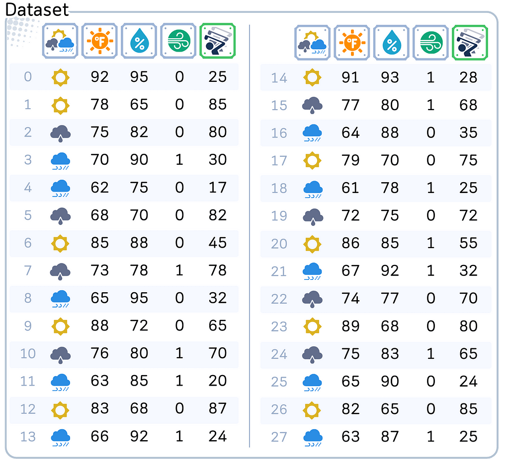

import pandas as pd
import numpy as np
from sklearn.model_selection import train_test_split

# Data preparation
dataset_dict = {
    'Outlook': ['sunny', 'sunny', 'overcast', 'rain', 'rain', 'overcast', 'sunny', 'overcast', 'rain', 'sunny', 'overcast', 'rain', 'sunny', 'rain',
                'sunny', 'overcast', 'rain', 'sunny', 'rain', 'overcast', 'sunny', 'rain', 'overcast', 'sunny', 'overcast', 'rain', 'sunny', 'rain'],
    'Temp.': [92.0, 78.0, 75.0, 70.0, 62.0, 68.0, 85.0, 73.0, 65.0, 88.0, 76.0, 63.0, 83.0, 66.0,
              91.0, 77.0, 64.0, 79.0, 61.0, 72.0, 86.0, 67.0, 74.0, 89.0, 75.0, 65.0, 82.0, 63.0],
    'Humid.': [95.0, 65.0, 82.0, 90.0, 75.0, 70.0, 88.0, 78.0, 95.0, 72.0, 80.0, 85.0, 68.0, 92.0,
               93.0, 80.0, 88.0, 70.0, 78.0, 75.0, 85.0, 92.0, 77.0, 68.0, 83.0, 90.0, 65.0, 87.0],
    'Wind': [False, False, False, True, False, False, False, True, False, False, True, True, False, True,
             True, True, False, False, True, False, True, True, False, False, True, False, False, True],
    'Num_Players': [25, 85, 80, 30, 17, 82, 45, 78, 32, 65, 70, 20, 87, 24,
                   28, 68, 35, 75, 25, 72, 55, 32, 70, 80, 65, 24, 85, 25]
}

# Data preprocessing
df = pd.DataFrame(dataset_dict)
df = pd.get_dummies(df, columns=['Outlook'], prefix='', prefix_sep='', dtype=int)
df['Wind'] = df['Wind'].astype(int)

This might sound simple, but there’s a catch. We only have information from 28 different days — that’s not a lot! And to make things even trickier, we need to split this data into two parts: 14 days to help our model learn (we call this training data), and 14 days to test if our model actually works (test data).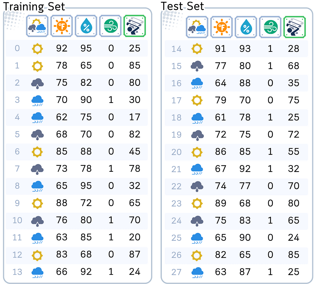

# Split features and target
X, y = df.drop('Num_Players', axis=1), df['Num_Players']
X_train, X_test, y_train, y_test = train_test_split(X, y, train_size=0.5, shuffle=False)

Think about how hard this is. There are so many possible combination of weather conditions. It can be sunny & humid, sunny & cool, rainy & windy, overcast & cool, or other combinations. With only 14 days of training data, we definitely won’t see every possible weather combination. But our model still needs to make good predictions for any weather condition it might encounter.

This is where our challenge begins. If we make our model too simple — like only looking at temperature — it will miss important details like wind and rain. That’s not good enough. But if we make it too complex — trying to account for every tiny weather change — it might think that one random quiet day during a rainy week means rain actually brings more players. With only 14 training examples, it’s easy for our model to get confused.

And here’s the thing: unlike many examples you see online, our data isn’t perfect. Some days might have similar weather but different player counts. Maybe there was a local event that day, or maybe it was a holiday — but our weather data can’t tell us that. This is exactly what makes real-world prediction problems tricky.

So before we get into building models, take a moment to appreciate what we’re trying to do:

Using just 14 examples to create a model that can predict player counts for ANY weather condition, even ones it hasn’t seen before.

This is the kind of real challenge that makes the bias-variance trade-off so important to understand.

Model Complexity

For our predictions, we’ll use decision tree regressors with varying depth (if you want to learn how this works, check out my article on decision tree basics). What matters for our discussion is how complex we let this model become.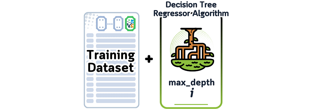

from sklearn.tree import DecisionTreeRegressor

# Define constants
RANDOM_STATE = 3 # As regression tree can be sensitive, setting this parameter assures that we always get the same tree
MAX_DEPTH = 5

# Initialize models
trees = {depth: DecisionTreeRegressor(max_depth=depth, random_state=RANDOM_STATE).fit(X_train, y_train) 
         for depth in range(1, MAX_DEPTH + 1)}

We’ll control the model’s complexity using its depth — from depth 1 (simplest) to depth 5 (most complex).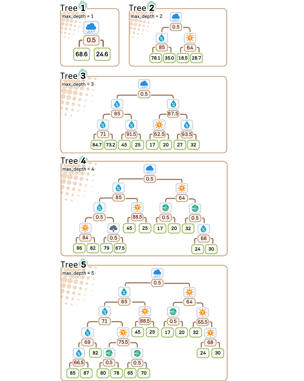

import matplotlib.pyplot as plt
from sklearn.tree import plot_tree

# Plot trees
for depth in range(1, MAX_DEPTH + 1):
    plt.figure(figsize=(12, 0.5*depth+1.5), dpi=300)
    plot_tree(trees[depth], feature_names=X_train.columns.tolist(), 
              filled=True, rounded=True, impurity=False, precision=1, fontsize=8)
    plt.title(f'Depth {depth}')
    plt.show()

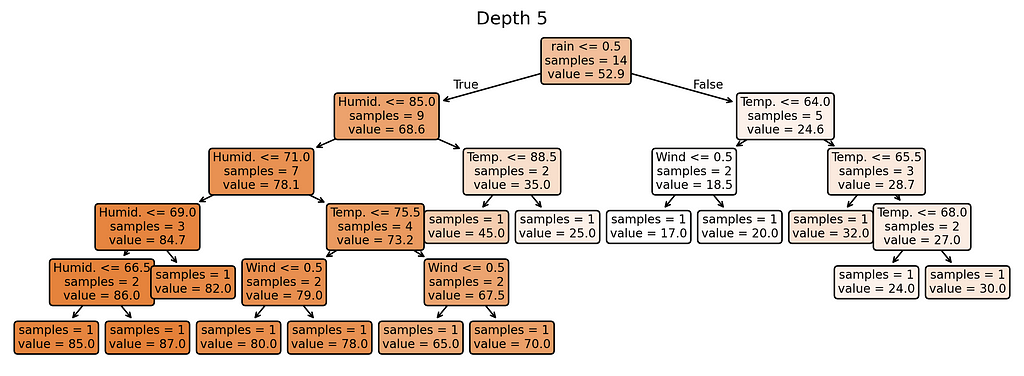
Why these complexity levels matter:

• Depth 1: Extremely simple — creates just a few different predictions
• Depth 2: Slightly more flexible — can create more varied predictions
• Depth 3: Moderate complexity — getting close to too many rules
• Depth 4–5: Highest complexity — nearly one rule per training example

Notice something interesting? Our most complex model (depth 5) creates almost as many different prediction rules as we have training examples. When a model starts making unique rules for almost every training example, it’s a clear sign we’ve made it too complex for our small dataset.

Throughout the next sections, we’ll see how these different complexity levels perform on our golf course data, and why finding the right complexity is crucial for making reliable predictions.

What Makes a Model “Good”?

Prediction Errors

The main goal in prediction is to make guesses as close to the truth as possible. We need a way to measure errors that sees guessing too high or too low as equally bad. A prediction 10 units above the real answer is just as wrong as one 10 units below it.

This is why we use Root Mean Square Error (RMSE) as our measurement. RMSE gives us the typical size of our prediction errors. If RMSE is 7, our predictions are usually off by about 7 units. If it’s 3, we’re usually off by about 3 units. A lower RMSE means better predictions.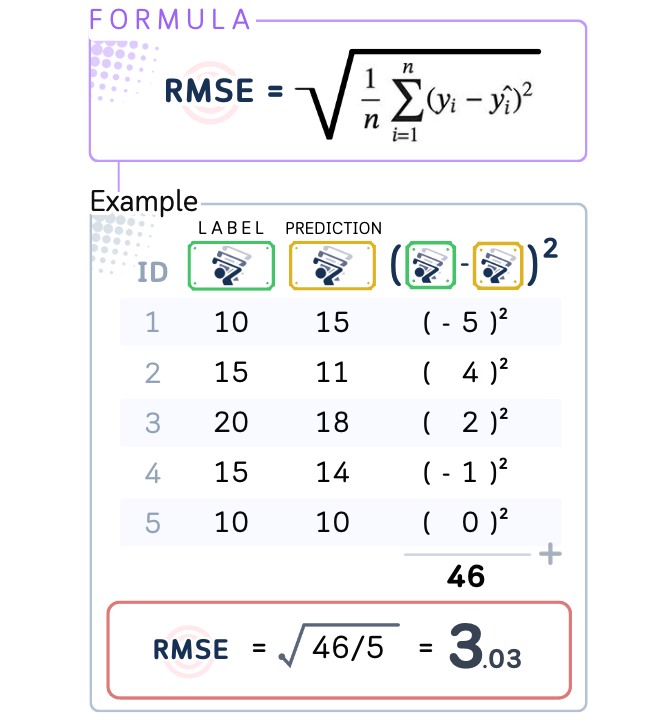

When measuring model performance, we always calculate two different errors. First is the training error — how well the model performs on the data it learned from. Second is the test error — how well it performs on new data it has never seen. This test error is crucial because it tells us how well our model will work in real-world situations where it faces new data.

⛳️ Looking at Our Golf Course Predictions

In our golf course case, we’re trying to predict daily player counts based on weather conditions. We have data from 28 different days, which we split into two equal parts:

• Training data: Records from 14 days that our model uses to learn patterns
• Test data: Records from 14 different days that we keep hidden from our model

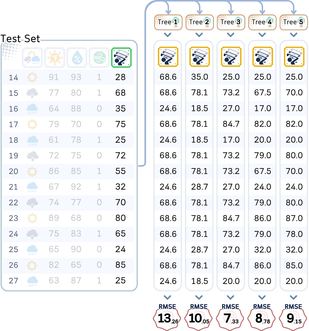
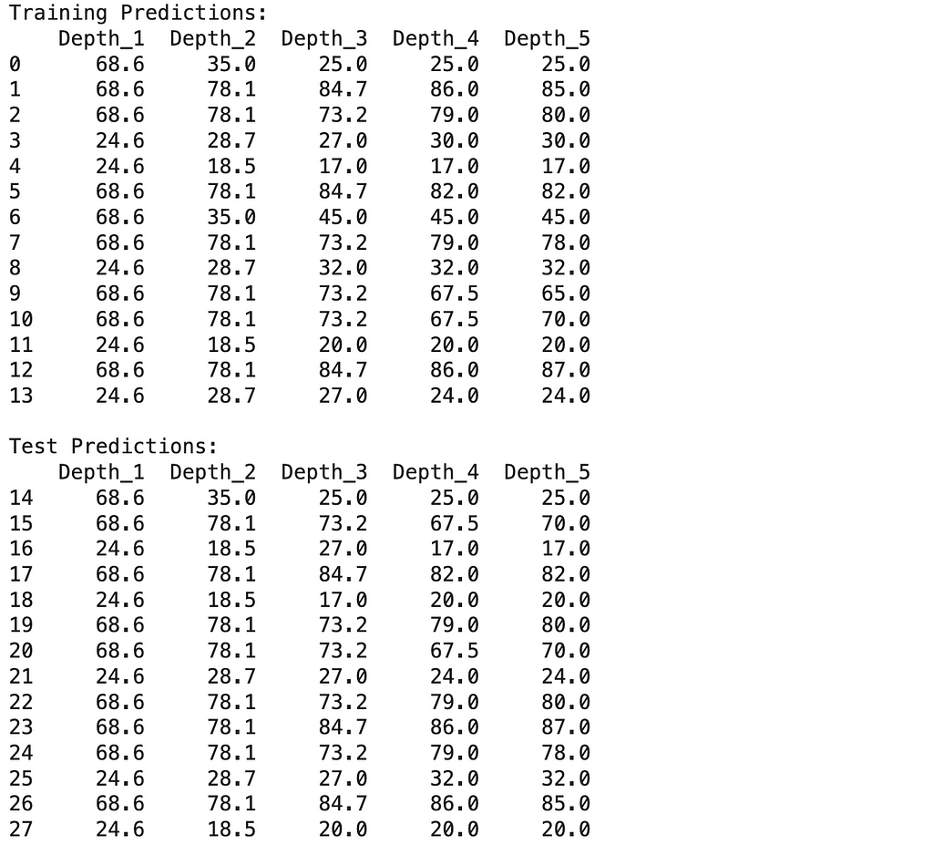
Using the models we made, let’s test both the training data and the test data, and also calculating their RMSE.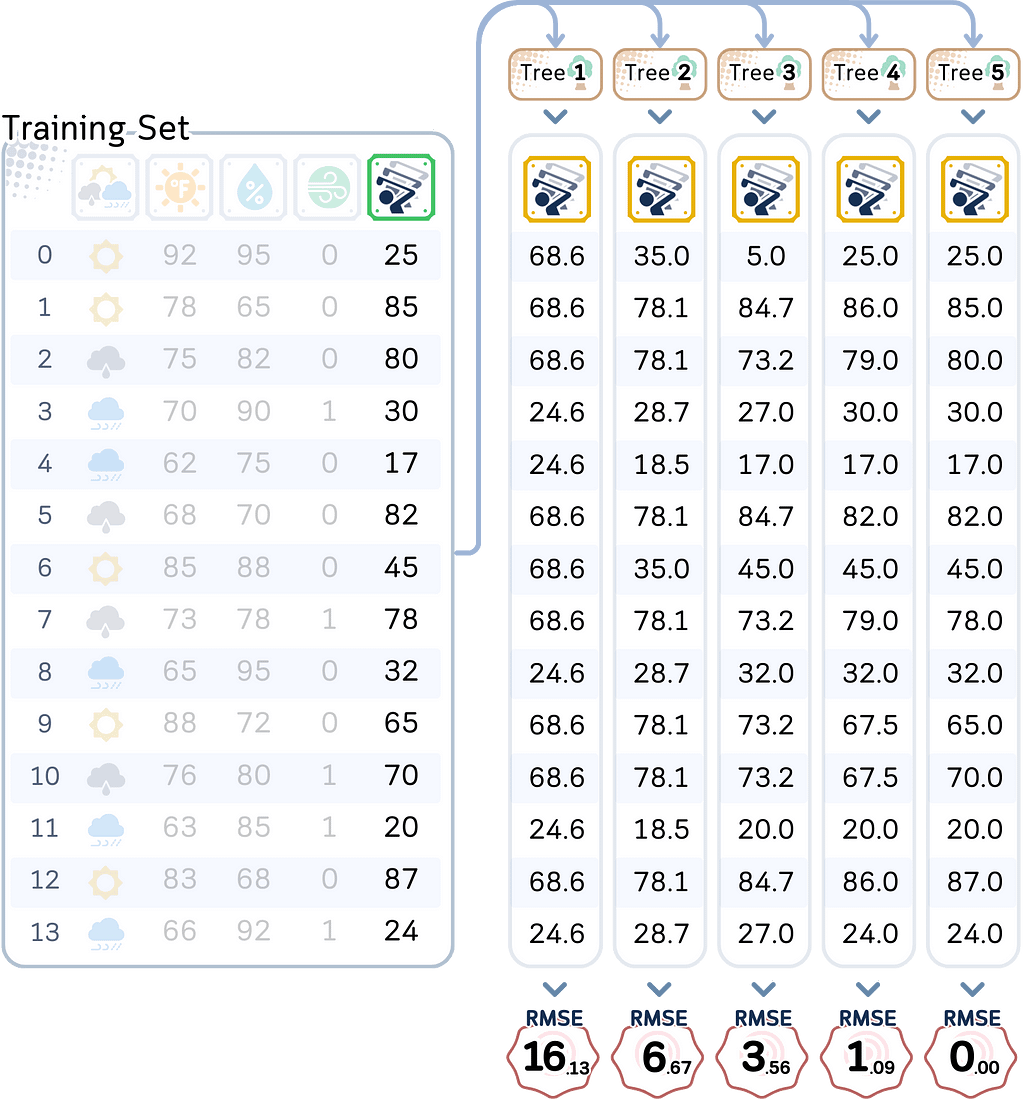

# Create training predictions DataFrame
train_predictions = pd.DataFrame({
    f'Depth_{i}': trees[i].predict(X_train) for i in range(1, MAX_DEPTH + 1)
})
#train_predictions['Actual'] = y_train.values
train_predictions.index = X_train.index

# Create test predictions DataFrame
test_predictions = pd.DataFrame({
    f'Depth_{i}': trees[i].predict(X_test) for i in range(1, MAX_DEPTH + 1)
})
#test_predictions['Actual'] = y_test.values
test_predictions.index = X_test.index

print("\nTraining Predictions:")
print(train_predictions.round(1))
print("\nTest Predictions:")
print(test_predictions.round(1))

from sklearn.metrics import root_mean_squared_error

# Calculate RMSE values
train_rmse = {depth: root_mean_squared_error(y_train, tree.predict(X_train))
              for depth, tree in trees.items()}
test_rmse = {depth: root_mean_squared_error(y_test, tree.predict(X_test))
             for depth, tree in trees.items()}

# Print RMSE summary as DataFrame
summary_df = pd.DataFrame({
    'Train RMSE': train_rmse.values(),
    'Test RMSE': test_rmse.values()
}, index=range(1, MAX_DEPTH + 1))
summary_df.index.name = 'max_depth'

print("\nSummary of RMSE values:")
print(summary_df.round(2))

Looking at these numbers, we can already see some interesting patterns: As we make our models more complex, they get better and better at predicting player counts for days they’ve seen before — to the point where our most complex model makes perfect predictions on training data.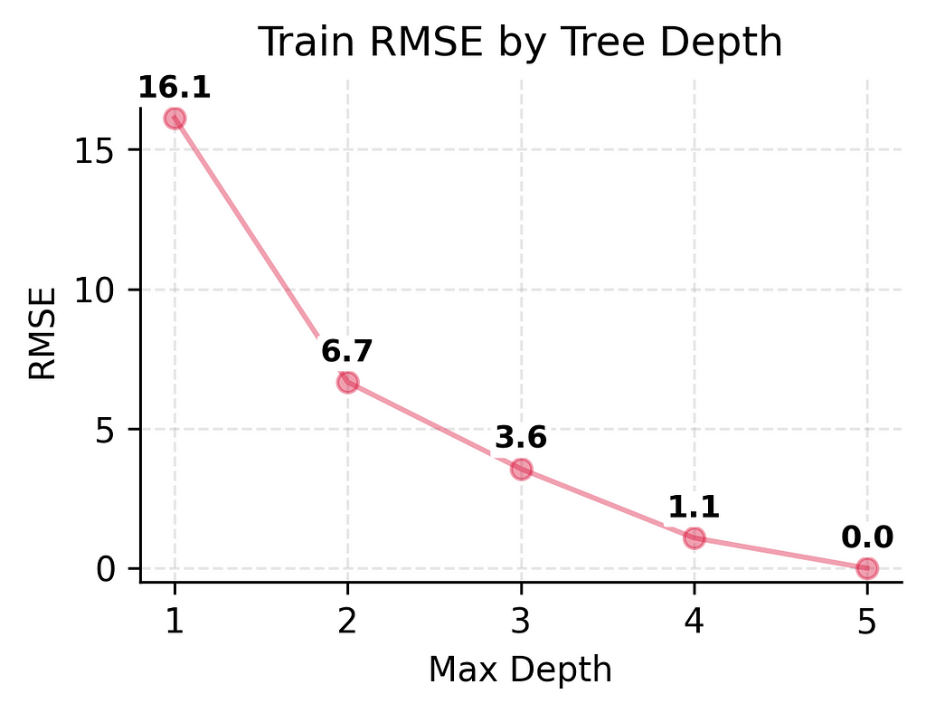

But the real test is how well they predict player counts for new days. Here, we see something different. While adding some complexity helps (the test error keeps getting better from depth 1 to depth 3), making the model too complex (depth 4–5) actually starts making things worse again.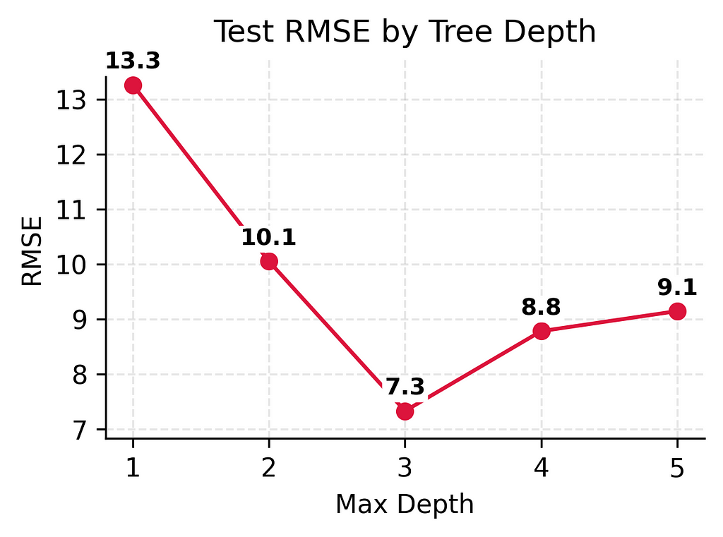

This difference between training and test performance (from being off by 3–4 players to being off by 9 players) shows a fundamental challenge in prediction: performing well on new, unseen situations is much harder than performing well on familiar ones. Even with our best performing model, we see this gap between training and test performance.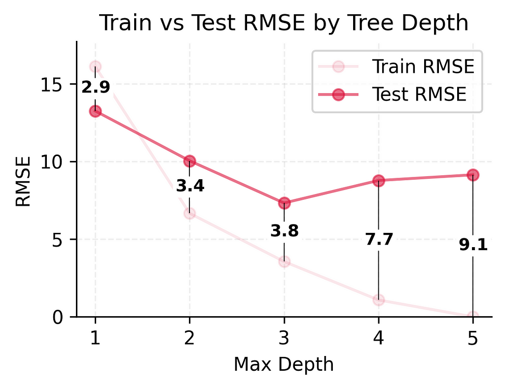

# Create figure
plt.figure(figsize=(4, 3), dpi=300)
ax = plt.gca()

# Plot main lines
plt.plot(summary_df.index, summary_df['Train RMSE'], marker='o', label='Train RMSE', 
         linestyle='-', color='crimson', alpha=0.1)
plt.plot(summary_df.index, summary_df['Test RMSE'], marker='o', label='Test RMSE', 
         linestyle='-', color='crimson', alpha=0.6)

# Add vertical lines and difference labels
for depth in summary_df.index:
    train_val = summary_df.loc[depth, 'Train RMSE']
    test_val = summary_df.loc[depth, 'Test RMSE']
    diff = abs(test_val - train_val)
    
    # Draw vertical line
    plt.vlines(x=depth, ymin=min(train_val, test_val), ymax=max(train_val, test_val), 
               colors='black', linestyles='-', lw=0.5)
    
    # Add white box behind text
    bbox_props = dict(boxstyle="round,pad=0.1", fc="white", ec="white")
    plt.text(depth - 0.15, (train_val + test_val) / 2, f'{diff:.1f}', 
             verticalalignment='center', fontsize=9, fontweight='bold',
             bbox=bbox_props)

# Customize plot
plt.xlabel('Max Depth')
plt.ylabel('RMSE')
plt.title('Train vs Test RMSE by Tree Depth')
plt.grid(True, linestyle='--', alpha=0.2)
plt.legend()

# Remove spines
ax.spines['top'].set_visible(False)
ax.spines['right'].set_visible(False)

# Set limits
plt.xlim(0.8, 5.2)
plt.ylim(0, summary_df['Train RMSE'].max() * 1.1)

plt.tight_layout()
plt.show()

Next, we’ll explore the two main ways models can fail: through consistently inaccurate predictions (bias) or through wildly inconsistent predictions (variance).

Understanding Bias (When Models Underfit)

What is Bias?

Bias happens when a model underfits the data by being too simple to capture important patterns. A model with high bias consistently makes large errors because it’s missing key relationships. Think of it as being consistently wrong in a predictable way.

When a model underfits, it shows specific behaviors:

• Similar sized errors across different predictions
• Training error is high
• Test error is also high
• Training and test errors are close to each other

High bias and underfitting are signs that our model needs to be more complex — it needs to pay attention to more patterns in the data. But how do we spot this problem? We look at both training and test errors. If both errors are high and similar to each other, we likely have a bias problem.

⛳️ Looking at Our Simple Golf Course Model

Let’s examine our simplest model’s performance (depth 1):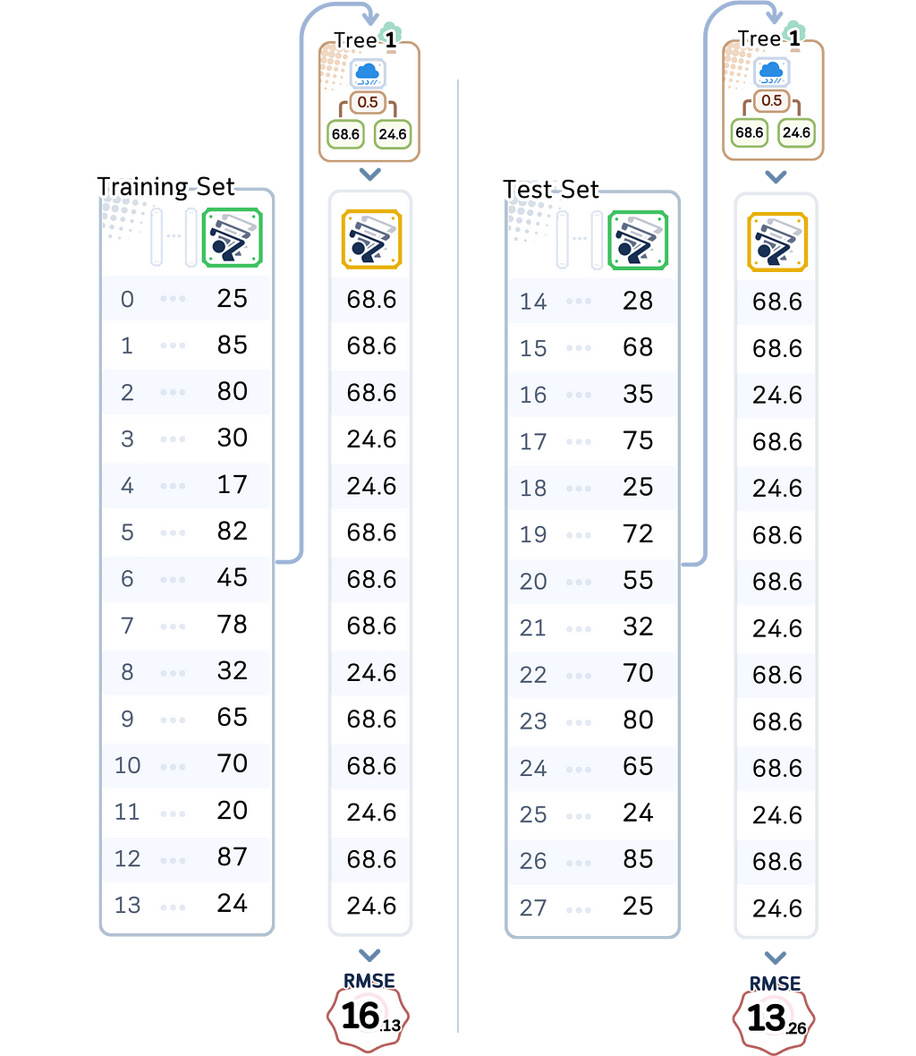

• Training RMSE: 16.13
  On average, it’s off by about 16 players even for days it trained on
• Test RMSE: 13.26
  For new days, it’s off by about 13 players

These numbers tell an important story. First, notice how high both errors are. Being off by 13–16 players is a lot when many days see between 20–80 players. Second, while the test error is higher (as we’d expect), both errors are notably large.

Looking deeper at what’s happening: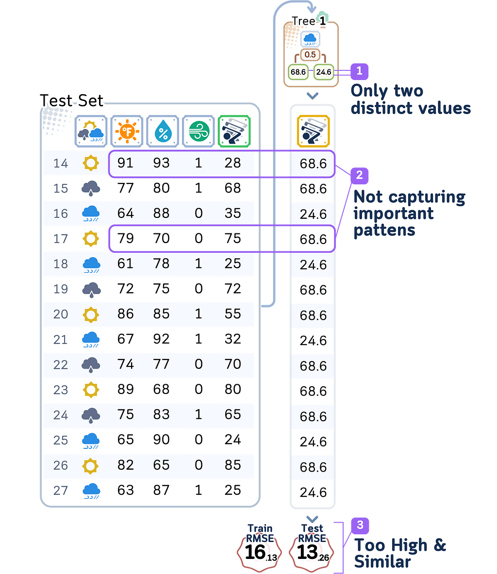

1. With depth 1, our model can only make one split decision. It might just split days based on whether it is raining or not, creating only two possible predictions for player counts. This means many different weather conditions get lumped together with the same prediction.
2. The errors follow clear patterns:
   - On hot, humid days: The model predicts too many players because it only sees whether it is raining or not
   - On cool, perfect days: The model predicts too few players because it ignores great playing conditions
3. Most telling is how similar the training and test errors are. Both are high, which means even when predicting days it trained on, the model does poorly. This is the clearest sign of high bias — the model is too simple to even capture the patterns in its training data.

This is the key problem with underfitting: the model lacks the complexity needed to capture important combinations of weather conditions that affect player turnout. Each prediction is wrong in predictable ways because the model simply can’t account for more than one weather factor at a time.

The solution seems obvious: make the model more complex so it can look at multiple weather conditions together. But as we’ll see in the next section, this creates its own problems.

Understanding Variance (When Models Overfit)

What is Variance?

Variance occurs when a model overfits by becoming too complex and overly sensitive to small changes in the data. While an underfit model ignores important patterns, an overfit model does the opposite — it treats every tiny detail as if it were an important pattern.

A model that’s overfitting shows these behaviors:

• Very small errors on training data
• Much larger errors on test data
• A big gap between training and test errors
• Predictions that change dramatically with small data changes

This problem is especially dangerous with small datasets. When we only have a few examples to learn from, an overfit model might perfectly memorize all of them without learning the true patterns that matter.

⛳️ Looking at Our Complex Golf Course Model

Let’s examine our most complex model’s performance (depth 5):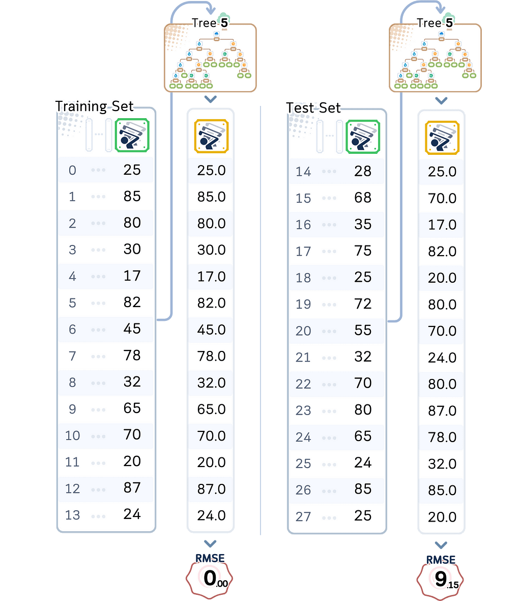

• Training RMSE: 0.00
  Perfect predictions! Not a single error on training data
• Test RMSE: 9.14
  But on new days, it’s off by about 9–10 players

These numbers reveal a classic case of overfitting. The training error of zero means our model learned to predict the exact number of players for every single day it trained on. Sounds great, right? But look at the test error — it’s much higher. This huge gap between training and test performance (from 0 to 9–10 players) is a red flag.

Looking deeper at what’s happening: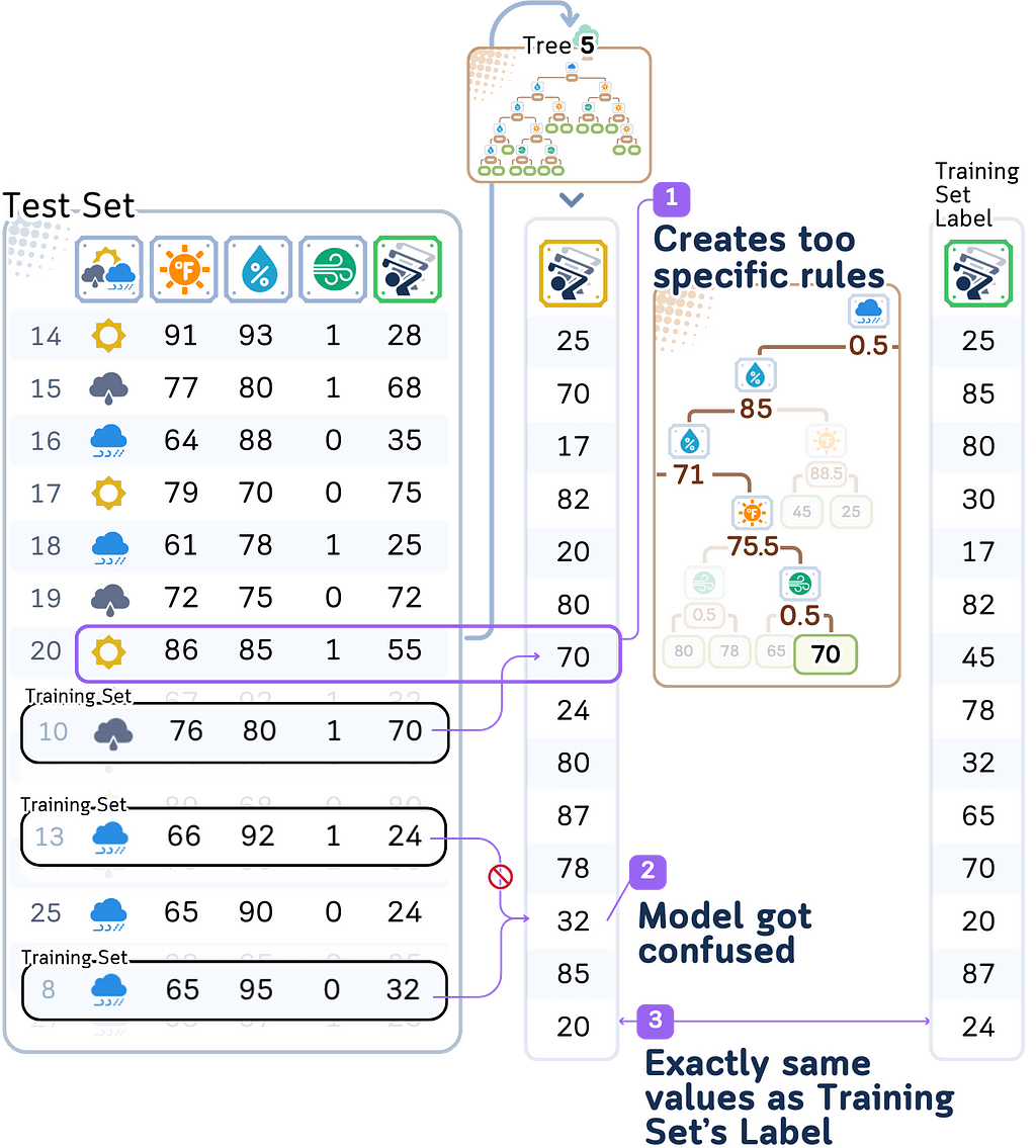

1. With depth 5, our model creates extremely specific rules. For example:
   - If it’s not rainy AND temperature is 76°F AND humidity is 80% AND it’s windy → predict exactly 70 players
   Each rule is based on just one or two days from our training data.
2. When the model sees slightly different conditions in the test data, it gets confused.
   This is very similar to our first rule above, but the model might predict a completely different number
3. With only 14 training examples, each training day gets its own highly specific set of rules. The model isn’t learning general patterns about how weather affects player counts — it’s just memorizing what happened on each specific day.

What’s particularly interesting is that while this overfit model does much better than our underfit model (test error 9.15), it’s actually worse than our moderately complex model. This shows how adding too much complexity can start hurting our predictions, even if the training performance looks perfect.

This is the fundamental challenge of overfitting: the model becomes so focused on making perfect predictions for the training data that it fails to learn the general patterns that would help it predict new situations well. It’s especially problematic when working with small datasets like ours, where creating a unique rule for each training example leaves us with no way to handle new situations reliably.

Finding the Balance

The Core Problem

Now we’ve seen both problems — underfitting and overfitting — let’s look at what happens when we try to fix them. This is where the real challenge of the bias-variance trade-off becomes clear.

Looking at our models’ performance as we made them more complex: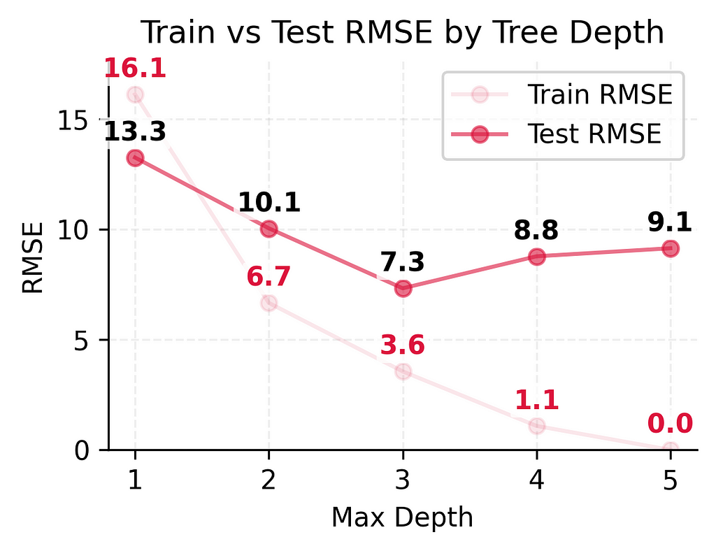

These numbers tell an important story. As we made our model more complex:

1. Training error kept getting better (16.3 → 6.7 → 3.6 → 1.1 → 0.0)
2. Test error improved significantly at first (13.3 → 10.1 → 7.3)
3. But then test error got slightly worse (7.3 → 8.8 → 9.1)

Why This Happens

This pattern isn’t a coincidence — it’s the fundamental nature of the bias-variance trade-off.

When we make a model more complex:

• It becomes less likely to underfit the training data (bias decreases)
• But it becomes more likely to overfit to small changes (variance increases)

Our golf course data shows this clearly:

1. The depth 1 model underfit badly — it could only split days into two groups, leading to large errors everywhere
2. Adding complexity helped — depth 2 could consider more weather combinations, and depth 3 found even better patterns
3. But depth 4 started to overfit — creating unique rules for nearly every training day

The sweet spot came with our depth 3 model: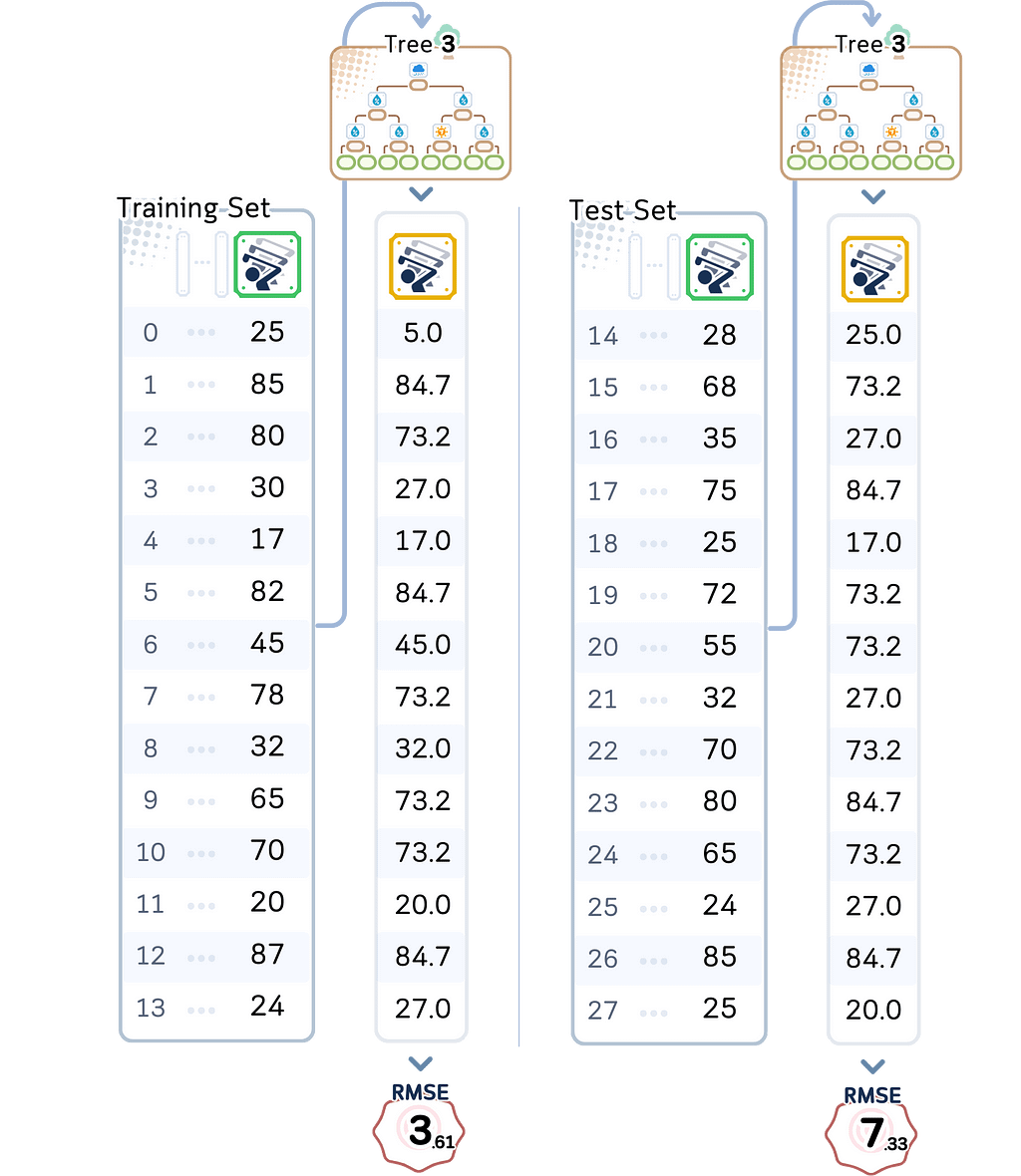

This model is complex enough to avoid underfitting while simple enough to avoid overfitting. It has the best test performance (RMSE 7.13) of all our models.

The Real-World Impact

With our golf course predictions, this trade-off has real consequences:

• Depth 1: Underfits by only looking at temperature, missing crucial information about rain or wind
• Depth 2: Can combine two factors, like temperature AND rain
• Depth 3: Can find patterns like “warm, low humidity, and not rainy means high turnout”
• Depth 4–5: Overfits with unreliable rules like “exactly 76°F with 80% humidity on a windy day means exactly 70 players”

This is why finding the right balance matters. With just 14 training examples, every decision about model complexity has big impacts. Our depth 3 model isn’t perfect — being off by 7 players on average isn’t ideal. But it’s much better than underfitting with depth 1 (off by 13 players) or overfitting with depth 4 (giving wildly different predictions for very similar weather conditions).

How to Choose the Right Balance

The Basic Approach

When picking the best model, looking at training and test errors isn’t enough. Why? Because our test data is limited — with only 14 test examples, we might get lucky or unlucky with how well our model performs on those specific days.

A better way to test our models is called cross-validation. Instead of using just one split of training and test data, we try different splits. Each time we:

1. Pick different samples as training data
2. Train our model
3. Test on the samples we didn’t use for training
4. Record the errors

By doing this multiple times, we can understand better how well our model really works.

⛳️ What We Found With Our Golf Course Data

Let’s look at how our different models performed across multiple training splits using cross-validation. Given our small dataset of just 14 training examples, we used K-fold cross-validation with k=7, meaning each validation fold had 2 samples.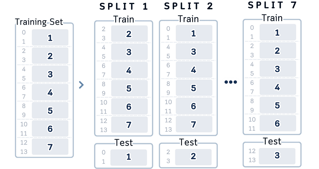

While this is a small validation size, it allows us to maximize our training data while still getting meaningful cross-validation estimates:

from sklearn.model_selection import KFold

def evaluate_model(X_train, y_train, X_test, y_test, n_splits=7, random_state=42):
   kf = KFold(n_splits=n_splits, shuffle=True, random_state=random_state)
   depths = range(1, 6)
   results = []
   
   for depth in depths:
       # Cross-validation scores
       cv_scores = []
       for train_idx, val_idx in kf.split(X_train):
           # Split data
           X_tr, X_val = X_train.iloc[train_idx], X_train.iloc[val_idx]
           y_tr, y_val = y_train.iloc[train_idx], y_train.iloc[val_idx]
           
           # Train and evaluate
           model = DecisionTreeRegressor(max_depth=depth, random_state=RANDOM_STATE)
           model.fit(X_tr, y_tr)
           val_pred = model.predict(X_val)
           cv_scores.append(np.sqrt(mean_squared_error(y_val, val_pred)))
       
       # Test set performance
       model = DecisionTreeRegressor(max_depth=depth, random_state=RANDOM_STATE)
       model.fit(X_train, y_train)
       test_pred = model.predict(X_test)
       test_rmse = np.sqrt(mean_squared_error(y_test, test_pred))
       
       # Store results
       results.append({
           'CV Mean RMSE': np.mean(cv_scores),
           'CV Std': np.std(cv_scores),
           'Test RMSE': test_rmse
       })
   
   return pd.DataFrame(results, index=pd.Index(depths, name='Depth')).round(2)

# Usage:
cv_df = evaluate_model(X_train, y_train, X_test, y_test)
print(cv_df)

Simple Model (depth 1):
- CV Mean RMSE: 20.28 (±12.90)
- Shows high variation in cross-validation (±12.90)
- Consistently poor performance across different data splits

Slightly Flexible Model (depth 2):
- CV Mean RMSE: 17.35 (±11.00)
- Lower average error than depth 1
- Still shows considerable variation in cross-validation
- Some improvement in predictive power

Moderate Complexity Model (depth 3):
- CV Mean RMSE: 16.16 (±9.26)
- More stable cross-validation performance
- Shows good improvement over simpler models
- Best balance of stability and accuracy

Complex Model (depth 4):
- CV Mean RMSE: 16.10 (±12.33)
- Very similar mean to depth 3
- Larger variation in CV suggests less stable predictions
- Starting to show signs of overfitting

Very Complex Model (depth 5):
- CV Mean RMSE: 16.59 (±11.73)
- CV performance starts to worsen
- High variation continues
- Clear sign of overfitting beginning to occur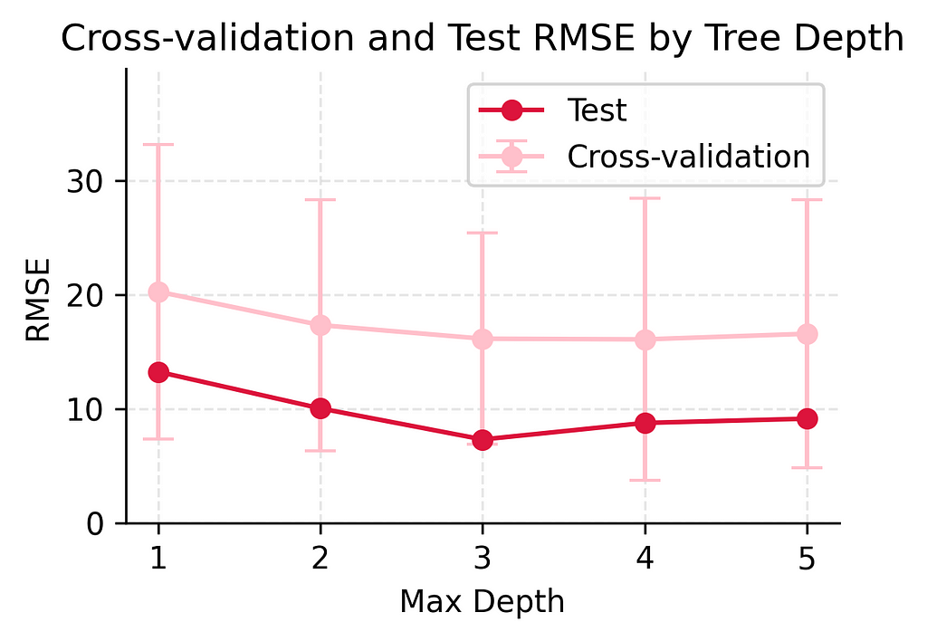

This cross-validation shows us something important: while our depth 3 model achieved the best test performance in our earlier analysis, the cross-validation results reveal that model performance can vary significantly. The high standard deviations (ranging from ±9.26 to ±12.90 players) across all models show that with such a small dataset, any single split of the data might give us misleading results. This is why cross-validation is so important — it helps us see the true performance of our models beyond just one lucky or unlucky split.

How to Make This Decision in Practice

Based on our results, here’s how we can find the right model balance:

1. Start Simple
   Start with the most basic model you can build. Check how well it works on both your training data and test data. If it performs poorly on both, that’s okay! It just means your model needs to be a bit more complex to capture the important patterns.
2. Gradually Add Complexity
   Now slowly make your model more sophisticated, one step at a time. Watch how the performance changes with each adjustment. When you see it starting to do worse on new data, that’s your signal to stop — you’ve found the right balance of complexity.
3. Watch for Warning Signs
   Keep an eye out for problems: If your model does extremely well on training data but poorly on new data, it’s too complex. If it does badly on all data, it’s too simple. If its performance changes a lot between different data splits, you’ve probably made it too complex.
4. Consider Your Data Size
   When you don’t have much data (like our 14 examples), keep your model simple. You can’t expect a model to make perfect predictions with very few examples to learn from. With small datasets, it’s better to have a simple model that works consistently than a complex one that’s unreliable.

Whenever we make prediction model, our goal isn’t to get perfect predictions — it’s to get reliable, useful predictions that will work well on new data. With our golf course dataset, being off by 6–7 players on average isn’t perfect, but it’s much better than being off by 11–12 players (too simple) or having wildly unreliable predictions (too complex).

Key Takeaways

Quick Ways to Spot Problems

Let’s wrap up what we’ve learned about building prediction models that actually work. Here are the key signs that tell you if your model is underfitting or overfitting: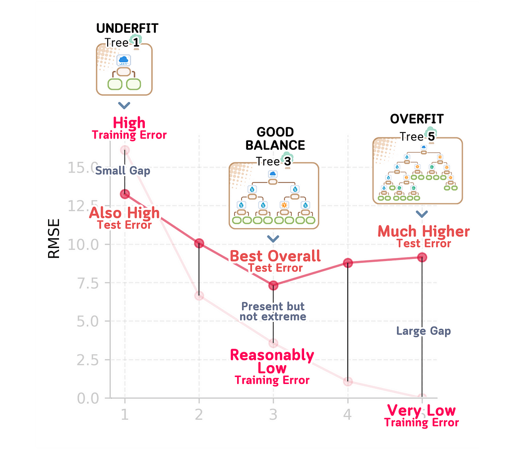

Signs of Underfitting (Too Simple):
When a model underfits, the training error will be high (like our depth 1 model’s 16.13 RMSE). Similarly, the test error will be high (13.26 RMSE). The gap between these errors is small (16.13 vs 13.26), which tells us that the model is always performing poorly. This kind of model is too simple to capture existing real relationships.

Signs of Overfitting (Too Complex):
An overfit model shows a very different pattern. You’ll see very low training error (like our depth 5 model’s 0.00 RMSE) but much higher test error (9.15 RMSE). This large gap between training and test performance (0.00 vs 9.15) is a sign that the model is easily distracted by noise in the training data and it is just memorizing the specific examples it was trained on.

Signs of a Good Balance (Like our depth 3 model):
A well-balanced model shows more promising characteristics. The training error is reasonably low (3.16 RMSE) and while the test error is higher (7.33 RMSE), it’s our best overall performance. The gap between training and test error exists but isn’t extreme (3.16 vs 7.33). This tells us the model has found the sweet spot: it’s complex enough to capture real patterns in the data while being simple enough to avoid getting distracted by noise. This balance between underfitting and overfitting is exactly what we’re looking for in a reliable model.

Final Remarks

The bias-variance trade-off isn’t just theory. It has real impacts on real predictions including in our golf course example before. The goal here isn’t to eliminate either underfitting or overfitting completely, because that’s impossible. What we want is to find the sweet spot where your model is complex enough to avoid underfitting and catch real patterns while being simple enough to avoid overfitting to random noise.

At the end, a model that’s consistently off by a little is often more useful than one that overfits — occasionally perfect but usually way off.

In the real world, reliability matters more than perfection.

Bias-Variance Tradeoff, Explained: A Visual Guide with Code Examples for Beginners was originally published in Towards Data Science on Medium, where people are continuing the conversation by highlighting and responding to this story.