Random Forest, Explained: A Visual Guide with Code Examples

ENSEMBLE LEARNING

Making tree-mendous predictions with random trees

Decision Tree Classifier, Explained: A Visual Guide with Code Examples for Beginners

Decision trees are a great starting point in machine learning — they’re clear and make sense. But there’s a catch: they often don’t work well when dealing with new data. The predictions can be inconsistent and unreliable, which is a real problem when you’re trying to build something useful.

This is where Random Forest comes in. It takes what’s good about decision trees and makes them work better by combining multiple trees together. It’s become a favorite tool for many data scientists because it’s both effective and practical.

Let’s see how Random Forest works and why it might be exactly what you need for your next project. It’s time to stop getting lost in the trees and see the forest for what it really is — your next reliable tool in machine learning.

Definition

A Random Forest is an ensemble machine learning model that combines multiple decision trees. Each tree in the forest is trained on a random sample of the data (bootstrap sampling) and considers only a random subset of features when making splits (feature randomization).

For classification tasks, the forest predicts by majority voting among trees, while for regression tasks, it averages the predictions. The model’s strength comes from its “wisdom of crowds” approach — while individual trees might make errors, the collective decision-making process tends to average out these mistakes and arrive at more reliable predictions.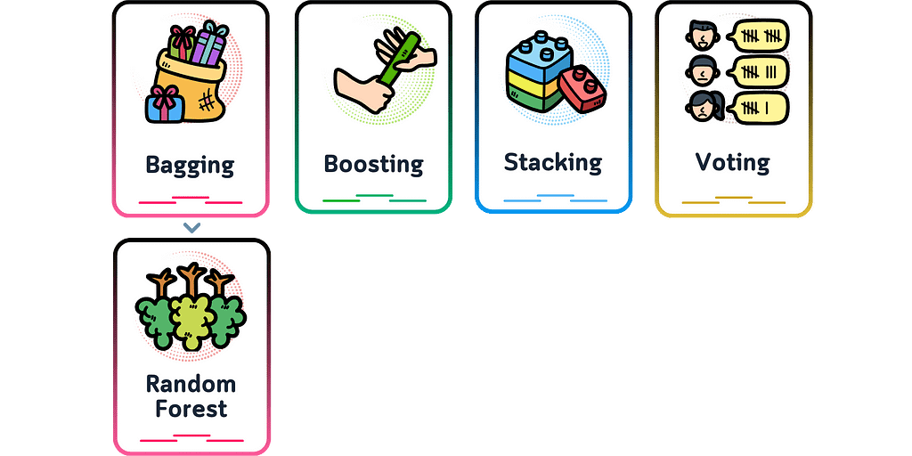

Dataset Used

Throughout this article, we’ll focus on the classic golf dataset as an example for classification. While Random Forests can handle both classification and regression tasks equally well, we’ll concentrate on the classification part — predicting whether someone will play golf based on weather conditions. The concepts we’ll explore can be easily adapted to regression problems (like predicting number of player) using the same principles.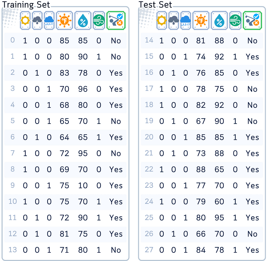

import pandas as pd
import numpy as np
from sklearn.model_selection import train_test_split

# Create and prepare dataset
dataset_dict = {
    'Outlook': ['sunny', 'sunny', 'overcast', 'rainy', 'rainy', 'rainy', 'overcast', 
                'sunny', 'sunny', 'rainy', 'sunny', 'overcast', 'overcast', 'rainy',
                'sunny', 'overcast', 'rainy', 'sunny', 'sunny', 'rainy', 'overcast',
                'rainy', 'sunny', 'overcast', 'sunny', 'overcast', 'rainy', 'overcast'],
    'Temperature': [85.0, 80.0, 83.0, 70.0, 68.0, 65.0, 64.0, 72.0, 69.0, 75.0, 75.0,
                   72.0, 81.0, 71.0, 81.0, 74.0, 76.0, 78.0, 82.0, 67.0, 85.0, 73.0,
                   88.0, 77.0, 79.0, 80.0, 66.0, 84.0],
    'Humidity': [85.0, 90.0, 78.0, 96.0, 80.0, 70.0, 65.0, 95.0, 70.0, 80.0, 70.0,
                 90.0, 75.0, 80.0, 88.0, 92.0, 85.0, 75.0, 92.0, 90.0, 85.0, 88.0,
                 65.0, 70.0, 60.0, 95.0, 70.0, 78.0],
    'Wind': [False, True, False, False, False, True, True, False, False, False, True,
             True, False, True, True, False, False, True, False, True, True, False,
             True, False, False, True, False, False],
    'Play': ['No', 'No', 'Yes', 'Yes', 'Yes', 'No', 'Yes', 'No', 'Yes', 'Yes', 'Yes',
             'Yes', 'Yes', 'No', 'No', 'Yes', 'Yes', 'No', 'No', 'No', 'Yes', 'Yes',
             'Yes', 'Yes', 'Yes', 'Yes', 'No', 'Yes']
}

# Prepare data
df = pd.DataFrame(dataset_dict)
df = pd.get_dummies(df, columns=['Outlook'], prefix='', prefix_sep='', dtype=int)
df['Wind'] = df['Wind'].astype(int)
df['Play'] = (df['Play'] == 'Yes').astype(int)

# Rearrange columns
column_order = ['sunny', 'overcast', 'rainy', 'Temperature', 'Humidity', 'Wind', 'Play']
df = df[column_order]

# Prepare features and target
X,y = df.drop('Play', axis=1), df['Play']
X_train, X_test, y_train, y_test = train_test_split(X, y, train_size=0.5, shuffle=False)

Main Mechanism

Here’s how Random Forest works:

1. Bootstrap Sampling: Each tree gets its own unique training set, created by randomly sampling from the original data with replacement. This means some data points may appear multiple times while others aren’t used.
2. Random Feature Selection: When making a split, each tree only considers a random subset of features (typically square root of total features).
3. Growing Trees: Each tree grows using only its bootstrap sample and selected features, making splits until it reaches a stopping point (like pure groups or minimum sample size).
4. Final Prediction: All trees vote together for the final prediction. For classification, take the majority vote of class predictions; for regression, average the predicted values from all trees.

Training Steps

The Random Forest algorithm constructs multiple decision trees and combines them. Here’s how it works:

Step 1: Bootstrap Sample Creation
1.0. Set the number of trees (default = 100)
1.1. For each tree in the forest:
a. Create new training set by random sampling original data with replacement until reaching original dataset size. This is called bootstrap sampling.
b. Mark and set aside non-selected samples as out-of-bag (OOB) samples for later error estimation

# Generate 100 bootstrap samples
n_samples = len(X_train)
n_bootstraps = 100
all_bootstrap_indices = []
all_oob_indices = []

np.random.seed(42)  # For reproducibility
for i in range(n_bootstraps):
    # Generate bootstrap sample indices
    bootstrap_indices = np.random.choice(n_samples, size=n_samples, replace=True)
    
    # Find OOB indices
    oob_indices = list(set(range(n_samples)) - set(bootstrap_indices))
    
    all_bootstrap_indices.append(bootstrap_indices)
    all_oob_indices.append(oob_indices)

# Print details for samples 1, 2, and 100
samples_to_show = [0, 1, 99]

for i in samples_to_show:
    print(f"\nBootstrap Sample {i+1}:")
    print(f"Chosen indices: {sorted(all_bootstrap_indices[i])}")
    print(f"Number of unique chosen indices: {len(set(all_bootstrap_indices[i]))}")
    print(f"OOB indices: {sorted(all_oob_indices[i])}")
    print(f"Number of OOB samples: {len(all_oob_indices[i])}")
    print(f"Percentage of OOB: {len(all_oob_indices[i])/n_samples*100:.1f}%")

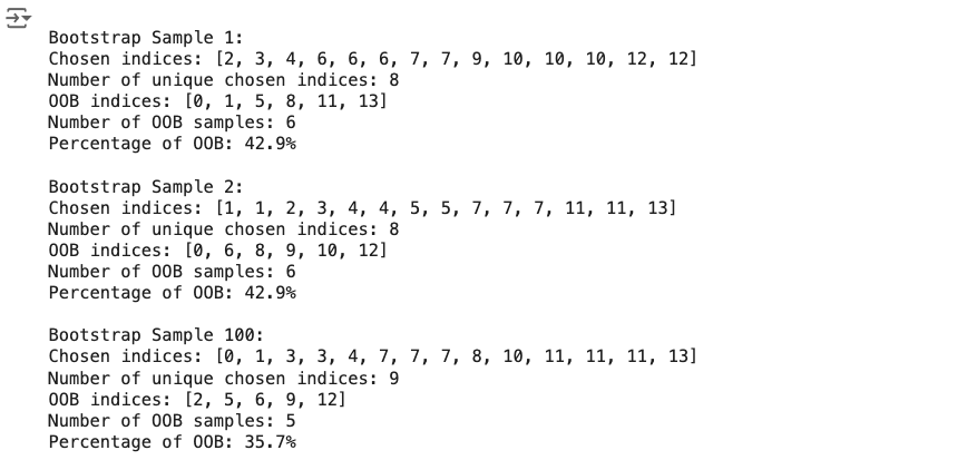
Notice how similar the percentages of OOB above? When doing bootstrap sampling of n samples, each individual sample has about a 37% chance of never being picked. This comes from the probability calculation (1–1/n)ⁿ, which approaches 1/e ≈ 0.368 as n gets larger. That’s why each tree ends up using roughly 63% of the data for training, with the remaining 37% becoming OOB samples.

Step 2: Tree Construction
2.1. Start at root node with complete bootstrap sample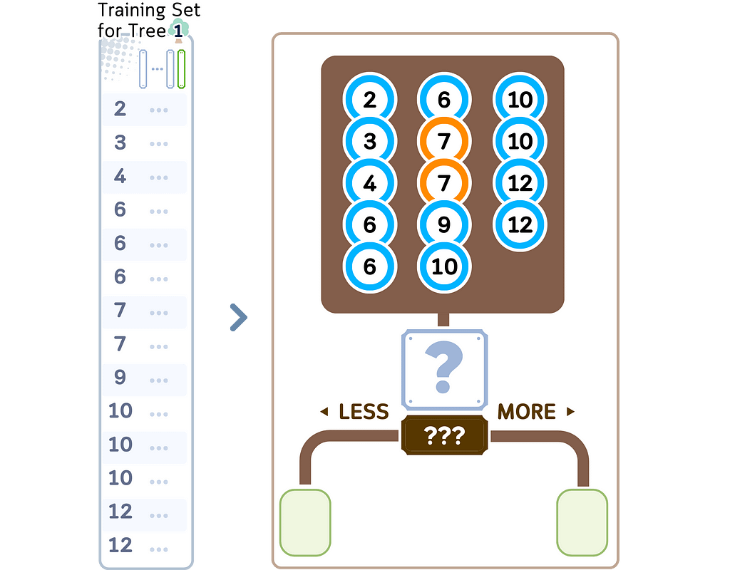

a. Calculate initial node impurity using all samples in node
· Classification: Gini or entropy
· Regression: MSE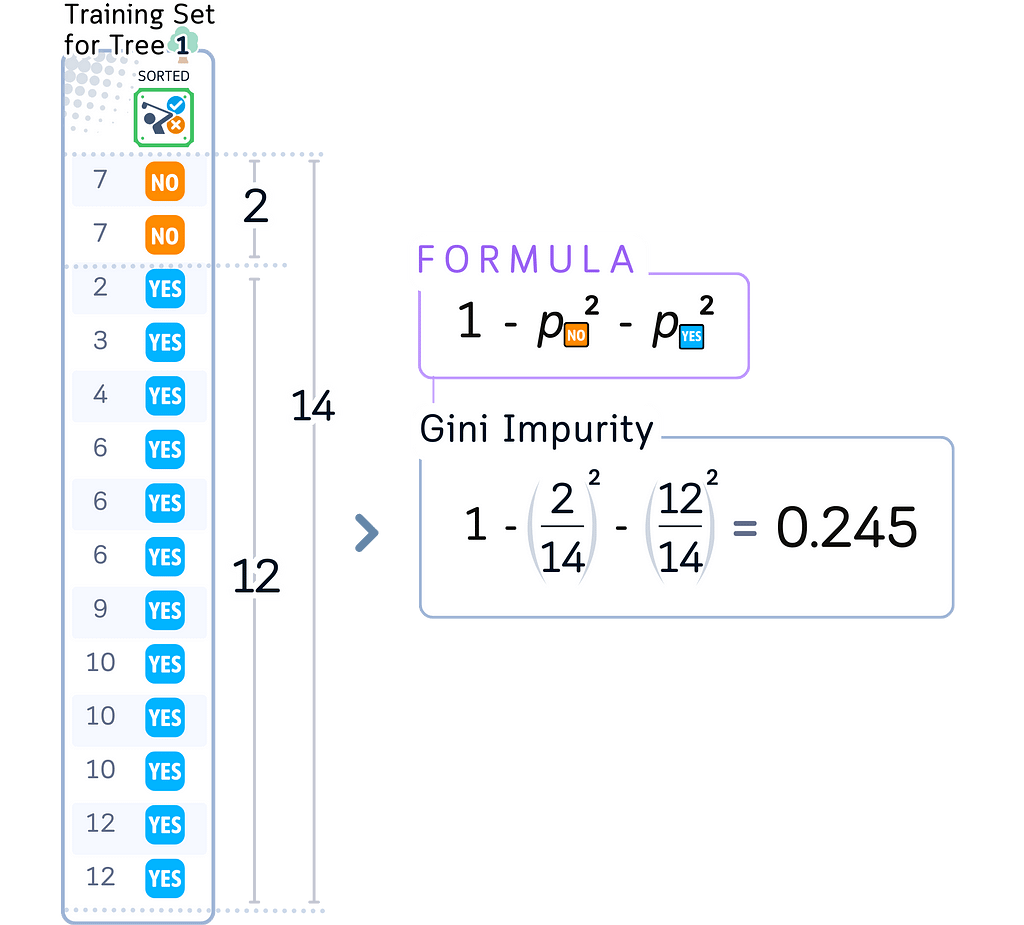

b. Select random subset of features from total available features:
· Classification: √n_features
· Regression: n_features/3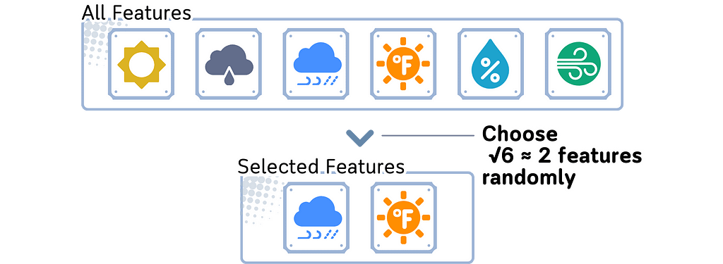

c. For each selected feature:
· Sort data points by feature values
· Identify potential split points (midpoints between consecutive unique feature values)

d. For each potential split point:
· Divide samples into left and right groups
· Calculate left child impurity using its samples
· Calculate right child impurity using its samples
· Calculate impurity reduction:
parent_impurity — (left_weight × left_impurity + right_weight × right_impurity)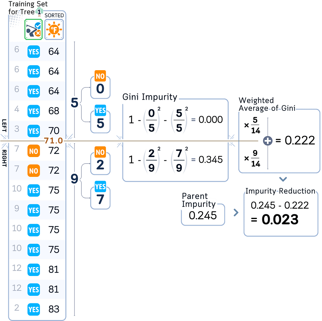

e. Split the current node data using the feature and split point that gives the highest impurity reduction. Then pass data points to the respective child nodes.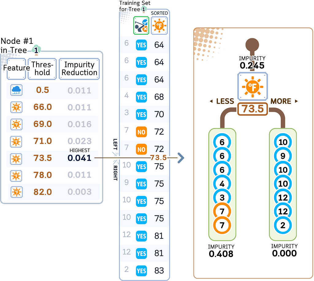

f. For each child node, repeat the process (step b-e) until:
- Pure node or minimum impurity decrease
- Minimum samples threshold
- Maximum depth
- Maximum leaf nodes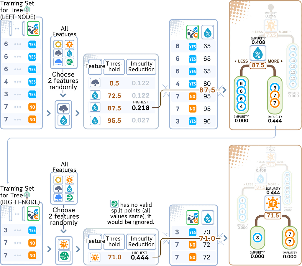

Step 3: Tree Construction
Repeat the whole Step 2 for other bootstrap samples.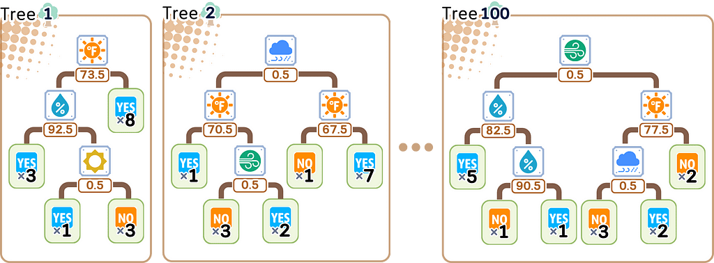

from sklearn.tree import plot_tree
from sklearn.ensemble import RandomForestClassifier

# Train Random Forest
np.random.seed(42)  # For reproducibility
rf = RandomForestClassifier(n_estimators=100, random_state=42)
rf.fit(X_train, y_train)

# Create visualizations for trees 1, 2, and 100
trees_to_show = [0, 1, 99]  # Python uses 0-based indexing
feature_names = X_train.columns.tolist()
class_names = ['No', 'Yes']

# Set up the plot
fig, axes = plt.subplots(1, 3, figsize=(20, 6), dpi=300)  # Reduced height, increased DPI
fig.suptitle('Decision Trees from Random Forest', fontsize=16)

# Plot each tree
for idx, tree_idx in enumerate(trees_to_show):
    plot_tree(rf.estimators_[tree_idx], 
              feature_names=feature_names,
              class_names=class_names,
              filled=True,
              rounded=True,
              ax=axes[idx],
              fontsize=10)  # Increased font size
    axes[idx].set_title(f'Tree {tree_idx + 1}', fontsize=12)

plt.tight_layout(rect=[0, 0.03, 1, 0.95])

Testing Step

For prediction, route new samples through all trees and aggregate:
- Classification: majority vote
- Regression: mean prediction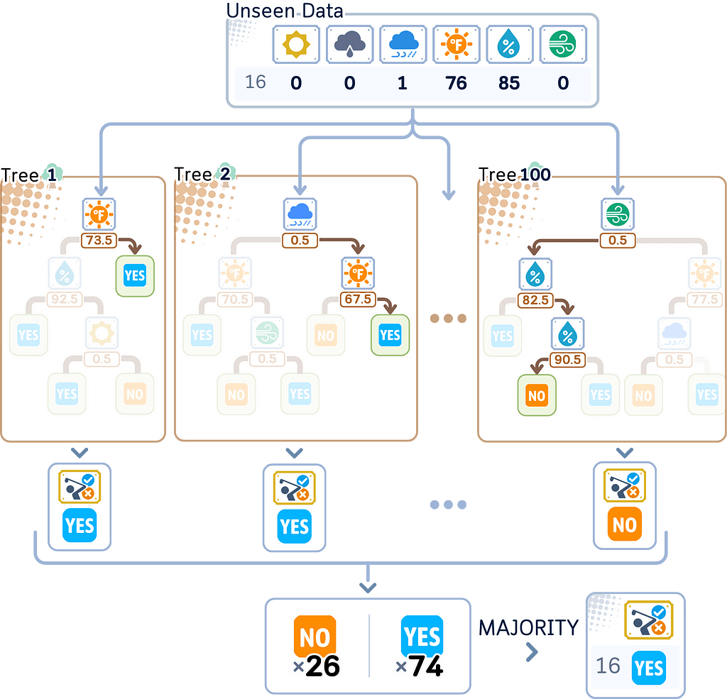

Out-of-Bag (OOB) Evaluation

Remember those samples that didn’t get used for training each tree — that leftover 1/3? Those are your OOB samples. Instead of just ignoring them, Random Forest uses them as a convenient validation set for each tree.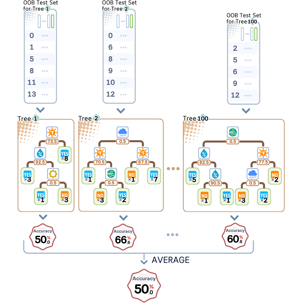

Evaluation Step

After building all the trees, we can evaluate the test set.

Key Parameters

The key Random Forest parameters (especially in scikit-learn) include all Decision Tree parameters, plus some unique ones.

Random Forest-specific parameters

• oob_score
  This uses leftover data (out-of-bag samples) to check how well the model works. This gives you a way to test your model without setting aside separate test data. It’s especially helpful with small datasets.
• n_estimators
  This parameter controls how many trees to build (default is 100).
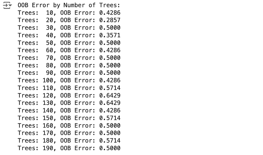
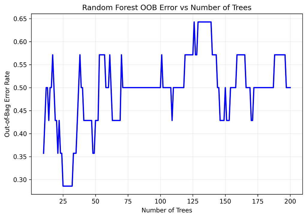
  To find the optimal number of trees, track the OOB error rate as you add more trees to the forest. The error typically drops quickly at first, then levels off. The point where it stabilizes suggests the optimal number — adding more trees after this gives minimal improvement while increasing computation time.

# Calculate OOB error for different numbers of trees
n_trees_range = range(10, 201)
oob_errors = [
    1 - RandomForestClassifier(n_estimators=n, oob_score=True, random_state=42).fit(X_train, y_train).oob_score_
    for n in n_trees_range
]

# Create a plot
plt.figure(figsize=(7, 5), dpi=300)
plt.plot(n_trees_range, oob_errors, 'b-', linewidth=2)
plt.xlabel('Number of Trees')
plt.ylabel('Out-of-Bag Error Rate')
plt.title('Random Forest OOB Error vs Number of Trees')
plt.grid(True, alpha=0.2)
plt.tight_layout()

# Print results at key intervals
print("OOB Error by Number of Trees:")
for i, error in enumerate(oob_errors, 1):
    if i % 10 == 0:
        print(f"Trees: {i:3d}, OOB Error: {error:.4f}")

• bootstrap
  This decides whether each tree learns from a random sample of data (True) or uses all data ( False). The default (True) helps create different kinds of trees, which is key to how Random Forests work. Only consider setting it to False when you have very little data and can’t afford to skip any samples.
• n_jobs
  This controls how many processor cores to use during training. Setting it to -1 uses all available cores, making training faster but using more memory. With big datasets, you might need to use fewer cores to avoid running out of memory.

Shared parameters with Decision Trees

The following parameters works the same way as in Decision Tree.

• max_depth: Maximum tree depth
• min_samples_split: Minimum samples needed to split a node
• min_samples_leaf: Minimum samples required at leaf node

Compared to Decision Tree, here are key differences in parameter importance:

1. max_depth
   This matters less in Random Forests because combining many trees helps prevent overfitting, even with deeper trees. You can usually let trees grow deeper to catch complex patterns in your data.
2. min_samples_split and min_samples_leaf
   These are less important in Random Forests because using many trees naturally helps avoid overfitting. You can usually set these to smaller numbers than you would with a single decision tree.

Pros & Cons

Pros:

1. Strong and Reliable: Random Forests give accurate results and are less likely to overfit than single decision trees. By using random sampling and mixing up which features each tree considers at each node, they work well across many problems without needing much adjustment.
2. Feature Importance: The model can tell you which features matter most in making predictions by measuring how much each feature helps across all trees. This helps you understand what drives your predictions.
3. Minimal Preprocessing: Random Forests handle both numerical and categorical variables well without much preparation. They work well with missing values and outliers, and can find complex relationships in your data automatically.

Cons:

1. Computational Cost: Training and using the model takes more time as you add more trees or make them deeper. While you can speed up training by using multiple processors, it still needs substantial computing power for big datasets.
2. Limited Interpretability: While you can see which features are important overall, it’s harder to understand exactly why the model made a specific prediction, unlike with single decision trees. This can be a problem when you need to explain each decision.
3. Prediction Speed: To make a prediction, data must go through all trees and then combine their answers. This makes Random Forests slower than simpler models, which might be an issue for real-time applications.

Final Remarks

I’ve grown to really like Random Forests after seeing how well they work in practice. By combining multiple trees and letting each one learn from different parts of the data, they consistently make better predictions — of course, more than using just one tree alone.

While you do need to adjust some settings like the number of trees, they usually perform well even without much fine-tuning. They do need more computing power (and sometimes struggle with rare cases in the data) but their reliable performance and ease of use make them my go-to choice for many projects. It’s clear why so many data scientists feel the same way!

???? Random Forest Classifier Code Summarized

import pandas as pd
import numpy as np
from sklearn.model_selection import train_test_split
from sklearn.metrics import accuracy_score
from sklearn.ensemble import RandomForestClassifier

# Create dataset
dataset_dict = {
    'Outlook': ['sunny', 'sunny', 'overcast', 'rainy', 'rainy', 'rainy', 'overcast', 
                'sunny', 'sunny', 'rainy', 'sunny', 'overcast', 'overcast', 'rainy',
                'sunny', 'overcast', 'rainy', 'sunny', 'sunny', 'rainy', 'overcast',
                'rainy', 'sunny', 'overcast', 'sunny', 'overcast', 'rainy', 'overcast'],
    'Temperature': [85.0, 80.0, 83.0, 70.0, 68.0, 65.0, 64.0, 72.0, 69.0, 75.0, 75.0,
                   72.0, 81.0, 71.0, 81.0, 74.0, 76.0, 78.0, 82.0, 67.0, 85.0, 73.0,
                   88.0, 77.0, 79.0, 80.0, 66.0, 84.0],
    'Humidity': [85.0, 90.0, 78.0, 96.0, 80.0, 70.0, 65.0, 95.0, 70.0, 80.0, 70.0,
                 90.0, 75.0, 80.0, 88.0, 92.0, 85.0, 75.0, 92.0, 90.0, 85.0, 88.0,
                 65.0, 70.0, 60.0, 95.0, 70.0, 78.0],
    'Wind': [False, True, False, False, False, True, True, False, False, False, True,
             True, False, True, True, False, False, True, False, True, True, False,
             True, False, False, True, False, False],
    'Play': ['No', 'No', 'Yes', 'Yes', 'Yes', 'No', 'Yes', 'No', 'Yes', 'Yes', 'Yes',
             'Yes', 'Yes', 'No', 'No', 'Yes', 'Yes', 'No', 'No', 'No', 'Yes', 'Yes',
             'Yes', 'Yes', 'Yes', 'Yes', 'No', 'Yes']
}

# Prepare data
df = pd.DataFrame(dataset_dict)
df = pd.get_dummies(df, columns=['Outlook'], prefix='', prefix_sep='', dtype=int)
df['Wind'] = df['Wind'].astype(int)
df['Play'] = (df['Play'] == 'Yes').astype(int)

# Rearrange columns
column_order = ['sunny', 'overcast', 'rainy', 'Temperature', 'Humidity', 'Wind', 'Play']
df = df[column_order]

# Split features and target
X, y = df.drop('Play', axis=1), df['Play']
X_train, X_test, y_train, y_test = train_test_split(X, y, train_size=0.5, shuffle=False)

# Train Random Forest
rf = RandomForestClassifier(n_estimators=100, max_features='sqrt', random_state=42)
rf.fit(X_train, y_train)

# Predict and evaluate
y_pred = rf.predict(X_test)
print(f"Accuracy: {accuracy_score(y_test, y_pred)}")

???? Random Forest Regressor Code Summarized

import pandas as pd
import numpy as np
from sklearn.model_selection import train_test_split
from sklearn.metrics import root_mean_squared_error
from sklearn.ensemble import RandomForestRegressor

# Create dataset
dataset_dict = {
    'Outlook': ['sunny', 'sunny', 'overcast', 'rain', 'rain', 'rain', 'overcast', 
                'sunny', 'sunny', 'rain', 'sunny', 'overcast', 'overcast', 'rain',
                'sunny', 'overcast', 'rain', 'sunny', 'sunny', 'rain', 'overcast',
                'rain', 'sunny', 'overcast', 'sunny', 'overcast', 'rain', 'overcast'],
    'Temp.': [85.0, 80.0, 83.0, 70.0, 68.0, 65.0, 64.0, 72.0, 69.0, 75.0, 75.0,
              72.0, 81.0, 71.0, 81.0, 74.0, 76.0, 78.0, 82.0, 67.0, 85.0, 73.0,
              88.0, 77.0, 79.0, 80.0, 66.0, 84.0],
    'Humid.': [85.0, 90.0, 78.0, 96.0, 80.0, 70.0, 65.0, 95.0, 70.0, 80.0, 70.0,
               90.0, 75.0, 80.0, 88.0, 92.0, 85.0, 75.0, 92.0, 90.0, 85.0, 88.0,
               65.0, 70.0, 60.0, 95.0, 70.0, 78.0],
    'Wind': [False, True, False, False, False, True, True, False, False, False, True,
             True, False, True, True, False, False, True, False, True, True, False,
             True, False, False, True, False, False],
    'Num_Players': [52, 39, 43, 37, 28, 19, 43, 47, 56, 33, 49, 23, 42, 13, 33, 29,
                    25, 51, 41, 14, 34, 29, 49, 36, 57, 21, 23, 41]
}

# Prepare data
df = pd.DataFrame(dataset_dict)
df = pd.get_dummies(df, columns=['Outlook'], prefix='', prefix_sep='')
df['Wind'] = df['Wind'].astype(int)

# Split features and target
X, y = df.drop('Num_Players', axis=1), df['Num_Players']
X_train, X_test, y_train, y_test = train_test_split(X, y, train_size=0.5, shuffle=False)

# Train Random Forest
rf = RandomForestRegressor(n_estimators=100, max_features='sqrt', random_state=42)
rf.fit(X_train, y_train)

# Predict and evaluate
y_pred = rf.predict(X_test)
rmse = root_mean_squared_error(y_test, y_pred)

print(f"Root Mean Squared Error: {rmse:.2f}")

Further Reading

For a detailed explanation of the RandomForestClassifier and RandomForestRegressor and its implementation in scikit-learn, readers can refer to the official documentation, which provides comprehensive information on its usage and parameters.

Technical Environment

This article uses Python 3.7 and scikit-learn 1.5. While the concepts discussed are generally applicable, specific code implementations may vary slightly with different versions.

About the Illustrations

Unless otherwise noted, all images are created by the author, incorporating licensed design elements from Canva Pro.

Random Forest, Explained: A Visual Guide with Code Examples was originally published in Towards Data Science on Medium, where people are continuing the conversation by highlighting and responding to this story.