Optimizing the Data Processing Performance in PySpark

PySpark techniques and strategies to tackle common performance challenges: A practical walkthrough

Apache Spark has been one of the leading analytical engines in recent years due to its power in distributed data processing. PySpark, the Python API for Spark, is often used for personal and enterprise projects to address data challenges. For example, we can efficiently implement feature engineering for time-series data using PySpark, including ingestion, extraction, and visualization. However, despite its capacity to handle large datasets, performance bottlenecks can still arise under various scenarios such as extreme data distribution and complex data transformation workflow.

This article will examine different common performance issues in data processing with PySpark on Databricks, and walk through various strategies for fine-tuning to achieve faster execution.

Imagine you open an online retail shop that offers a variety of products and is primarily targeted at U.S. customers. You plan to analyze buying habits from current transactions to satisfy more needs of current customers and serve more new ones. This motivates you to put much effort into processing the transaction records as a preparation step.

#0 Mock data

We first simulate 1 million transaction records (surely expected to handle much larger datasets in real big data scenarios) in a CSV file. Each record includes a customer ID, product purchased, and transaction details such as payment methods and total amounts. One note worth mentioning is that a product agent with customer ID #100 has a significant customer base, and thus occupies a significant portion of purchases in your shop for drop-shipping.

Below are the codes demonstrating this scenario:

import csv
import datetime
import numpy as np
import random

# Remove existing ‘retail_transactions.csv’ file, if any
! rm -f /p/a/t/h retail_transactions.csv

# Set the no of transactions and othet configs
no_of_iterations = 1000000
data = []
csvFile = 'retail_transactions.csv'

# Open a file in write mode
with open(csvFile, 'w', newline='') as f:
 
   fieldnames = ['orderID', 'customerID', 'productID', 'state', 'paymentMthd', 'totalAmt', 'invoiceTime']
   writer = csv.DictWriter(f, fieldnames=fieldnames)
   writer.writeheader()
 
   for num in range(no_of_iterations):
     # Create a transaction record with random values
     new_txn = {
     'orderID': num,
     'customerID': random.choice([100, random.randint(1, 100000)]),
     'productID': np.random.randint(10000, size=random.randint(1, 5)).tolist(),
     'state': random.choice(['CA', 'TX', 'FL', 'NY', 'PA', 'OTHERS']),
     'paymentMthd': random.choice(['Credit card', 'Debit card', 'Digital wallet', 'Cash on delivery', 'Cryptocurrency']),
     'totalAmt': round(random.random() * 5000, 2),
     'invoiceTime': datetime.datetime.now().isoformat()
     }
 
     data.append(new_txn)

  writer.writerows(data)

After mocking the data, we load the CSV file into the PySpark DataFrame using Databrick’s Jupyter Notebook.

# Set file location and type
file_location = "/FileStore/tables/retail_transactions.csv"
file_type = "csv"

# Define CSV options
schema = "orderID INTEGER, customerID INTEGER, productID INTEGER, state STRING, paymentMthd STRING, totalAmt DOUBLE, invoiceTime TIMESTAMP"
first_row_is_header = "true"
delimiter = ","

# Read CSV files into DataFrame
df = spark.read.format(file_type) \
  .schema(schema) \
  .option("header", first_row_is_header) \
  .option("delimiter", delimiter) \
  .load(file_location)

We additionally create a reusable decorator utility to measure and compare the execution time of different approaches within each function.

import time

# Measure the excution time of a given function
def time_decorator(func):
  def wrapper(*args, **kwargs):
    begin_time = time.time()
    output = func(*args, **kwargs)
    end_time = time.time()
    print(f"Execution time of function {func.__name__}: {round(end_time - begin_time, 2)} seconds.")
  return output
return wrapper

Okay, all the preparation is completed. Let’s explore different potential challenges of execution performance in the following sections.

#1 Storage

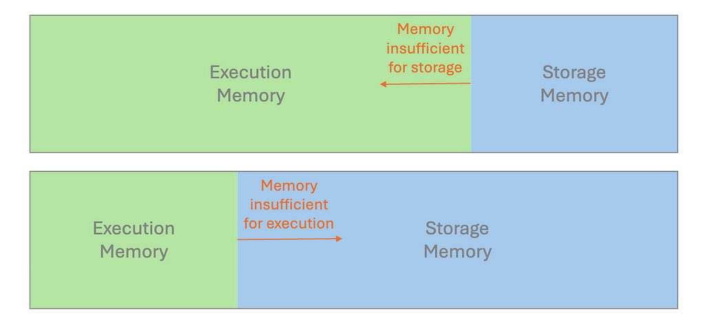
Spark uses Resilient Distributed Dataset (RDD) as its core building blocks, with data typically kept in memory by default. Whether executing computations (like joins and aggregations) or storing data across the cluster, all operations contribute to memory usage in a unified region.

If we design improperly, the available memory may become insufficient. This causes excess partitions to spill onto the disk, which results in performance degradation.

Caching and persisting intermediate results or frequently accessed datasets are common practices. While both cache and persist serve the same purposes, they may differ in their storage levels. The resources should be used optimally to ensure efficient read and write operations.

For example, if transformed data will be reused repeatedly for computations and algorithms across different subsequent stages, it is advisable to cache that data.

Code example: Assume we want to investigate different subsets of transaction records using a digital wallet as the payment method.

• Inefficient — Without caching

from pyspark.sql.functions import col

@time_decorator
def without_cache(data):
  # 1st filtering
  df2 = data.where(col("paymentMthd") == "Digital wallet")
  count = df2.count()

  # 2nd filtering
  df3 = df2.where(col("totalAmt") > 2000)
  count = df3.count()
    
  return count

display(without_cache(df))

• Efficient — Caching on a critical dataset

from pyspark.sql.functions import col

@time_decorator
def after_cache(data):
  # 1st filtering with cache
  df2 = data.where(col("paymentMthd") == "Digital wallet").cache()
  count = df2.count()

  # 2nd filtering
  df3 = df2.where(col("totalAmt") > 2000)
  count = df3.count()
    
  return count

display(after_cache(df))

After caching, even if we want to filter the transformed dataset with different transaction amount thresholds or other data dimensions, the execution times will still be more manageable.

#2 Shuffle

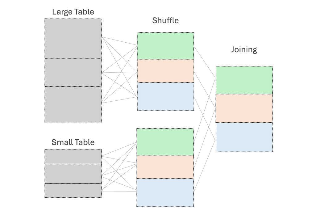
When we perform operations like joining DataFrames or grouping by data fields, shuffling occurs. This is necessary to redistribute all records across the cluster and to ensure those with the same key are on the same node. This in turn facilitates simultaneous processing and combining of the results.

However, this shuffle operation is costly — high execution times and additional network overhead due to data movement between nodes.

To reduce shuffling, there are several strategies:

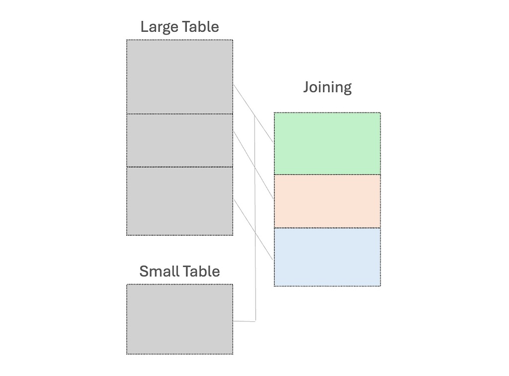
(1) Use broadcast variables for the small dataset, to send a read-only copy to every worker node for local processing

While “small” dataset is often defined by a maximum memory threshold of 8GB per executor, the ideal size for broadcasting should be determined through experimentation on specific case.

(2) Early filtering, to minimize the amount of data processed as early as possible; and

(3) Control the number of partitions to ensure optimal performance

Code examples: Assume we want to return the transaction records that match our list of states, along with their full names

• Inefficient — shuffle join between a large dataset and a small one

from pyspark.sql.functions import col

@time_decorator
def no_broadcast_var(data):
  # Create small dataframe
  small_data = [("CA", "California"), ("TX", "Texas"), ("FL", "Florida")]
  small_df = spark.createDataFrame(small_data, ["state", "stateLF"])

  # Perform joining
  result_no_broadcast = data.join(small_df, "state")

  return result_no_broadcast.count()

display(no_broadcast_var(df))

• Efficient — join the large dataset with the small one using a broadcast variable

from pyspark.sql.functions import col, broadcast

@time_decorator
def have_broadcast_var(data):
  small_data = [("CA", "California"), ("TX", "Texas"), ("FL", "Florida")]
  small_df = spark.createDataFrame(small_data, ["state", "stateFullName"])

  # Create broadcast variable and perform joining
  result_have_broadcast = data.join(broadcast(small_df), "state")

  return result_have_broadcast.count()

display(have_broadcast_var(df))

#3 Skewness

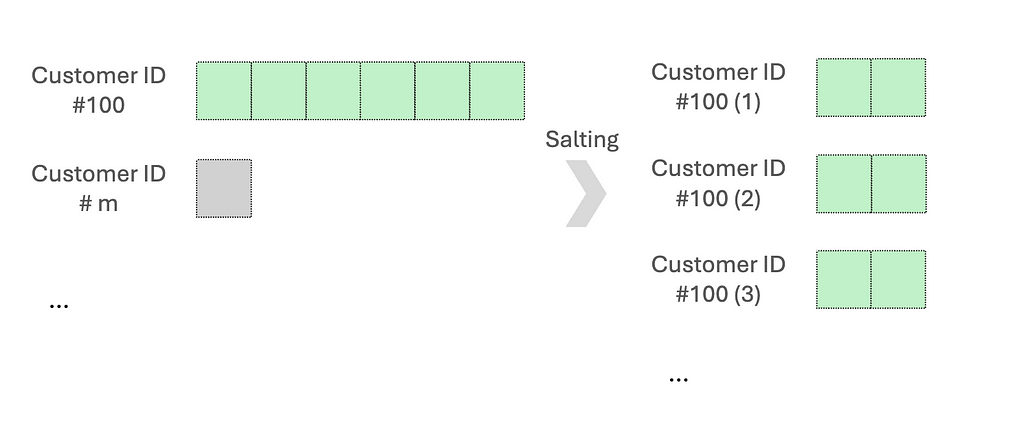
Data can sometimes be unevenly distributed, especially for data fields used as the key for processing. This leads to imbalanced partition sizes, in which some partitions are significantly larger or smaller than the average.

Since the execution performance is limited by the longest-running tasks, it is necessary to address the over-burdened nodes.

One common approach is salting. This works by adding randomized numbers to the skewed key so that there is a more uniform distribution across partitions. Let’s say when aggregating data based on the skewed key, we will aggregate using the salted key and then aggregate with the original key. Another method is re-partitioning, which increases the number of partitions to help distribute the data more evenly.

Code examples: We want to aggregate an asymmetric dataset, mainly skewed by customer ID #100.

• Inefficient — directly use the skewed key

from pyspark.sql.functions import col, desc

@time_decorator
def no_salting(data):
  # Perform aggregation
  agg_data = data.groupBy("customerID").agg({"totalAmt": "sum"}).sort(desc("sum(totalAmt)"))
  return agg_data

display(no_salting(df))

• Efficient — use the salting skewed key for aggregation

from pyspark.sql.functions import col, lit, concat, rand, split, desc

@time_decorator
def have_salting(data):
  # Salt the customerID by adding the suffix
  salted_data = data.withColumn("salt", (rand() * 8).cast("int")) \
                .withColumn("saltedCustomerID", concat(col("customerID"), lit("_"), col("salt")))

  # Perform aggregation
 agg_data = salted_data.groupBy("saltedCustomerID").agg({"totalAmt": "sum"})

 # Remove salt for further aggregation
 final_result = agg_data.withColumn("customerID", split(col("saltedCustomerID"), "_")[0]).groupBy("customerID").agg({"sum(totalAmt)": "sum"}).sort(desc("sum(sum(totalAmt))"))

 return final_result

display(have_salting(df))

A random prefix or suffix to the skewed keys will both work. Generally, 5 to 10 random values are a good starting point to balance between spreading out the data and maintaining high complexity.

#4 Serialization

People often prefer using user-defined functions (UDFs) since it is flexible in customizing the data processing logic. However, UDFs operate on a row-by-row basis. The code shall be serialized by the Python interpreter, sent to the executor JVM, and then deserialized. This incurs high serialization costs and prevents Spark from optimizing and processing the code efficiently.

The simple and direct approach is to avoid using UDFs when possible.

We should first consider using the built-in Spark functions, which can handle tasks such as aggregation, arrays/maps operations, date/time stamps, and JSON data processing. If the built-in functions do not satisfy your desired tasks indeed, we can consider using pandas UDFs. They are built on top of Apache Arrow for lower overhead costs and higher performance, compared to UDFs.

Code examples: The transaction price is discounted based on the originating state.

• Inefficient — using a UDF

from pyspark.sql.functions import udf
from pyspark.sql.types import DoubleType
from pyspark.sql import functions as F
import numpy as np

# UDF to calculate discounted amount
def calculate_discount(state, amount):
  if state == "CA":
    return amount * 0.90  # 10% off
  else:
    return amount * 0.85  # 15% off

discount_udf = udf(calculate_discount, DoubleType())

@time_decorator
def have_udf(data):
  # Use the UDF
  discounted_data = data.withColumn("discountedTotalAmt", discount_udf("state", "totalAmt"))

  # Show the results
  return discounted_data.select("customerID", "totalAmt", "state", "discountedTotalAmt").show()

display(have_udf(df))

• Efficient — using build-in PySpark functions

from pyspark.sql.functions import when

@time_decorator
def no_udf(data):
  # Use when and otherwise to discount the amount based on conditions 
  discounted_data = data.withColumn(
  "discountedTotalAmt",
  when(data.state == "CA", data.totalAmt * 0.90)  # 10% off
  .otherwise(data.totalAmt * 0.85))  # 15% off

  # Show the results
  return discounted_data.select("customerID", "totalAmt", "state", "discountedTotalAmt").show()

display(no_udf(df))

In this example, we use the built-in PySpark functions “when and otherwise” to effectively check multiple conditions in sequence. There are unlimited examples based on our familiarity with those functions. For instance, pyspark.sql.functions.transforma function that aids in applying a transformation to each element in the input array has been introduced since PySpark version 3.1.0.

#5 Spill

As discussed in the Storage section, a spill occurs by writing temporary data from memory to disk due to insufficient memory to hold all the required data. Many performance issues we have covered are related to spills. For example, operations that shuffle large amounts of data between partitions can easily lead to memory exhaustion and subsequent spill.

It is crucial to examine the performance metrics in Spark UI. If we discover the statistics for Spill(Memory) and Spill(Disk), the spill is probably the reason for long-running tasks. To remediate this, try to instantiate a cluster with more memory per worker, e.g. increase the executor process size, by tuning the configuration value spark.executor.memory; Alternatively, we can configure spark.memory.fraction to adjust how much memory is allocated for execution and storage.

Wrapping it Up

We came across several common factors leading to performance degradation in PySpark, and the possible improvement methods:

• Storage: use cache and persist to store the frequently used intermediate results
• Shuffle: use broadcast variables for a small dataset to facilitate Spark’s local processing
• Skewness: execute salting or repartitioning to distribute the skewed data more uniformly
• Serialization: prefer to use built-in Spark functions to optimize the performance
• Spill: adjust the configuration value to allocate memory wisely

Recently, Adaptive Query Execution (AQE) has been newly addressed for dynamic planning and re-planning of queries based on runtime stats. This supports different features of query re-optimization that occur during query execution, which creates a great optimization technique. However, understanding data characteristics during the initial design is still essential, as it informs better strategies for writing effective codes and queries while using AQE for fine-tuning.

Before you go

If you enjoy this reading, I invite you to follow my Medium page and LinkedIn page. By doing so, you can stay updated with exciting content related to data science side projects, Machine Learning Operations (MLOps) demonstrations, and project management methodologies.

• Simplifying the Python Code for Data Engineering Projects
• Feature Engineering for Time-Series Using PySpark on Databricks

Optimizing the Data Processing Performance in PySpark was originally published in Towards Data Science on Medium, where people are continuing the conversation by highlighting and responding to this story.